Basic point cloud manipulation and visualization

Published: March 28, 2018 / Last updated: December 7, 2018

Tested on Matlab r2017b, GNU Octave 4.4.1

Setup

Download and uncompress the Digital Forestry Toolbox (DFT) Zip or Tar archive
Download the zh_2014_a.laz file from the DFT Zenodo repository and uncompress it with LASzip
Start Matlab/Octave
Delete any previous versions of the toolbox
Add the DFT folders to the Matlab/Octave search path using addpath(genpath('path to DFT main folder'))
Open dft_tutorial_1.m (located in the tutorials folder)

Step 1 - Reading the LAS file

We start by reading the LAS file using LASread():

pc = LASread('zh_2014_a.las');

Note that the point classification uses the following scheme:

Class	Description
2	Terrain
3	Low vegetation (< 50 cm)
4	Medium vegetation (< 3 m)
5	High vegetation (> 3 m)
6	Buildings
7	Outliers and incorrect measurements (Noise)
10	Bridges (> 3m)
12	Strip border points (Overlap)
15	Overhead lines, masts, antennae
17	Other (vehicles, etc. )

Step 2 - Subsetting

We now subset the point cloud to keep only medium and high vegetation points located within a Region Of Interest (ROI):

% define a Region Of Interest (ROI)
x_roi = [2699597, 2699584, 2699778, 2699804];
y_roi = [1271166, 1271307, 1271341, 1271170];

% create ROI logical index (with inclusion test)
idxl_roi = inpolygon(pc.record.x, pc.record.y, x_roi, y_roi);

% create class subset logical index
idxl_class = ismember(pc.record.classification, [4,5]);

% combine subsetting indices
idxl_sample = idxl_roi & idxl_class;

% apply subsetting indices
xyz_s = [pc.record.x(idxl_sample), pc.record.y(idxl_sample), pc.record.z(idxl_sample)];
intensity_s = pc.record.intensity(idxl_sample);

Step 3 - Visualization

Use scatter3() to create an interactive 3D plot of the point cloud subset created in the previou step. You can use caxis() to specify the colormap range and increase contrast. Also note that it may useful to specify opengl hardware at the beginning of your script, for better graphics performance when working with large datasets.

figure
scatter3(xyz_s(:,1), ...
xyz_s(:,2), ...
xyz_s(:,3), ...
6, ...
intensity_s, ...
'Marker', '.');
colorbar
caxis(quantile(intensity_s, [0.01, 0.99]))
axis equal tight
title('Return intensity')
xlabel('x')
ylabel('y')
ylabel('z')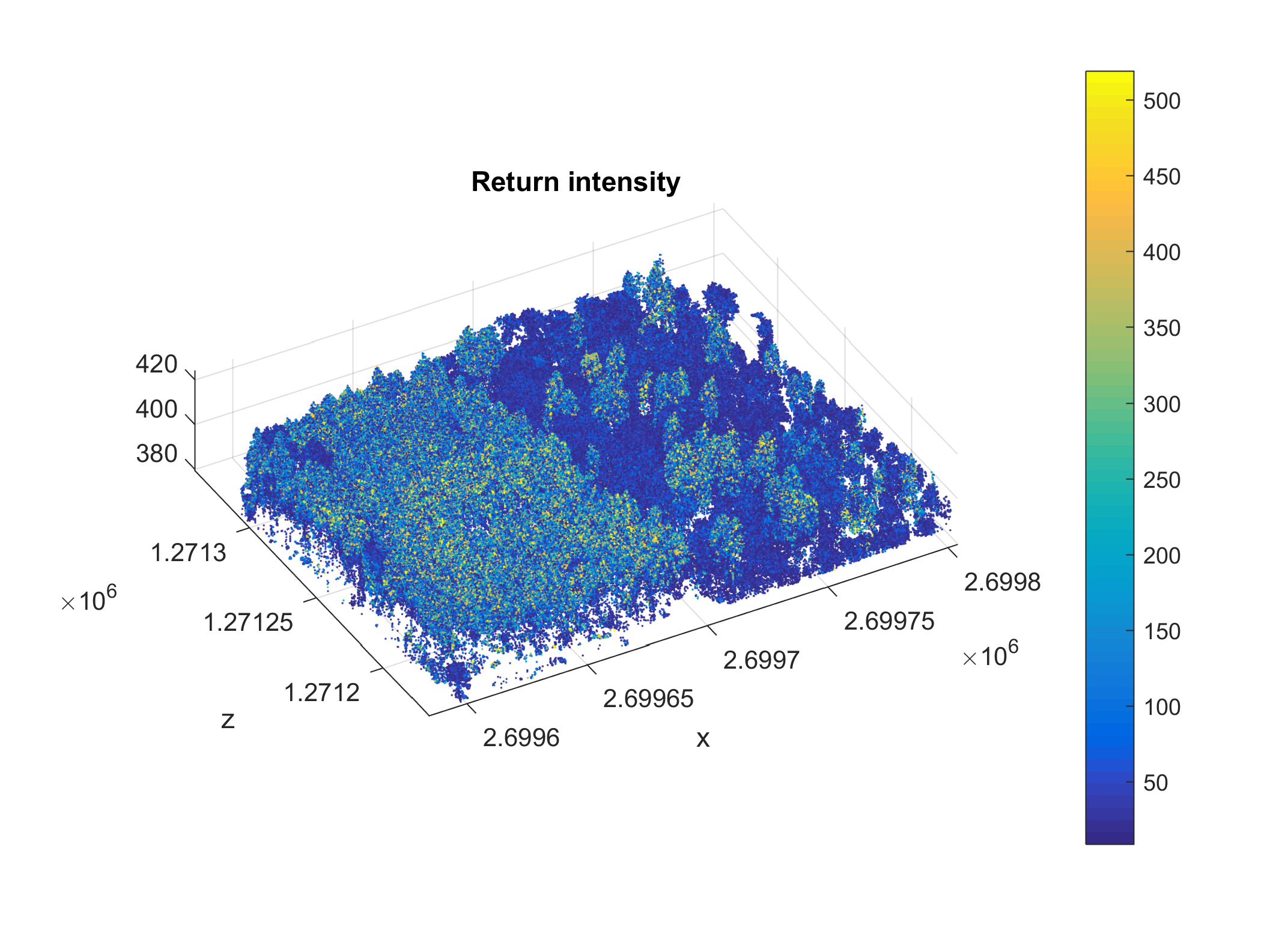

Figure 1 - Point cloud subset colored by return intensity. Notice the intensity difference between coniferous and deciduous trees (the point cloud was acquired in leaf-off conditions, in March 2014).

Step 4 - Checking the acquisition dates

Knowing when the data you are using was acquired is important to identify the phenological stage and to correlate your analysis with field observations. Four time formats are commonly encountered when working with airborne laser scanning data:

Format	Description
GPS week time	The fractional number of seconds since the beginning of the GPS week.
Standard GPS time	The fractional number of seconds since January 6, 1980 00:00h. Since it is not affected by leap seconds, Standard GPS time is now ahead of UTC time by several seconds.
Adjusted Standard GPS Time	Standard GPS time minus 10⁹ (for improved floating point resolution).
Coordinated Universal Time (UTC)	International time standard, also known as Greenwich Mean Time (GMT).

The ASPRS LAS format can store the GPS timestamp of each point in either GPS week time or adjusted standard GPS time. The time format is specified in the LAS file header Global Encoding field (starting with version LAS 1.2). In Matlab, you can check its value in pc.header.global_encoding_gps_time_type. The dataset we are using now is in LAS 1.1 format which does not provide any metadata on the time format. Nonetheless, the range of values in the GPS time record indicates it is stored in Adjusted Standard GPS Time. Thus, to get the UTC time, you can use:

utc_time = gps2utc(pc.record.gps_time + 10^9, 'verbose', true);

You'll notice the dataset was acquired on March 10 and 13, 2014.

Step 5 - Clipping directly to a LAS file

You may want to clip a LAS file and directly write it to a new file. You can do this with LASclip():

LASclip('zh_2014_a.las', ...
       [x_roi', y_roi'], ...
       'zh_2014_a_clip.las', ...
       'verbose', true);

Step 6 - Computing the spatial extent of a LAS file (Matlab only)

You can compute the spatial extent (bounding box, convex hull or concave hull) of LAS files with LASextent():

extent = LASextent('zh_2014_a.las', ...
    'zh_2014_a_extent.shp', ...
    'method', 'convexhull', ...
    'fig', false, ...
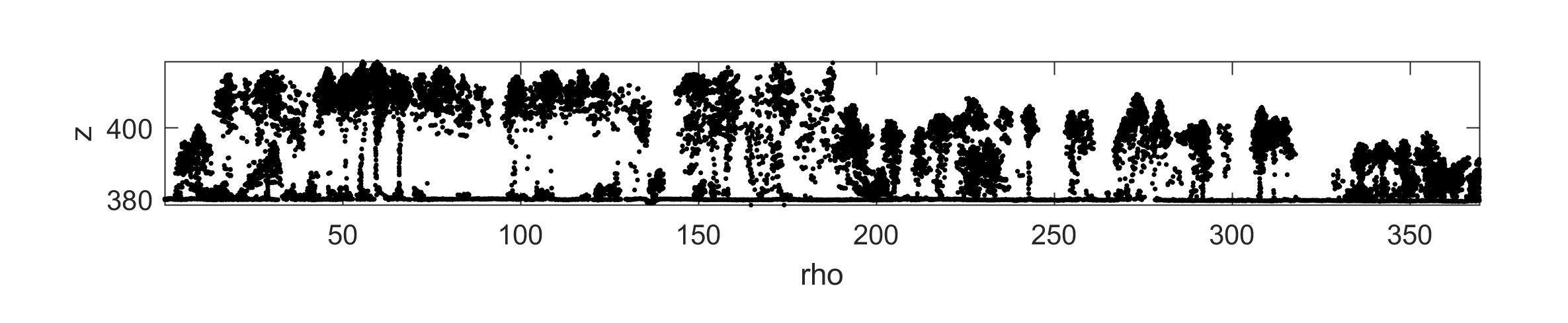
    'verbose', true);

Step 7 - Extracting a cross-section from a 3D point cloud

You can extract cross-sections of 3D point clouds with crossSection():

width = 2;
p0 = [2699582, 1271120];
p1 = [2699884, 1271333];
[~, ~, profile] = crossSection([pc.record.x, pc.record.y, pc.record.z], ...
    width, ...
    p0, ...
    p1, ...
    'verbose', true, ...
    'fig', true);

The resulting cross section should look like this:

Digital-Forestry-Toolbox