Individual tree crown detection using marker controlled watershed segmentation
Published: May 15, 2018 / Last updated: April 4, 2021
Tested on Matlab r2020b, GNU Octave 6.2.0
Setup
- Download and uncompress the Digital Forestry Toolbox (DFT) Zip or Tar archive
- Download the zh_2014_a.laz file from the DFT Zenodo repository and uncompress it with LASzip
- Start Matlab/Octave
- Delete any previous versions of the toolbox
- Add the DFT folders to the Matlab/Octave search path using
addpath(genpath('path to DFT main folder')) - Open
dft_tutorial_2.m(located in the tutorials folder)
Step 1 - Reading the LAS file
We start by reading the LAS file using LASread():
pc = LASread('zh_2014_a.las');Note that the point classification uses the following scheme:
| Class | Description |
|---|---|
| 2 | Terrain |
| 3 | Low vegetation (< 50 cm) |
| 4 | Medium vegetation (< 3 m) |
| 5 | High vegetation (> 3 m) |
| 6 | Buildings |
| 7 | Outliers and incorrect measurements (Noise) |
| 10 | Bridges (> 3m) |
| 12 | Strip border points (Overlap) |
| 15 | Overhead lines, masts, antennae |
| 17 | Other (vehicles, etc. ) |
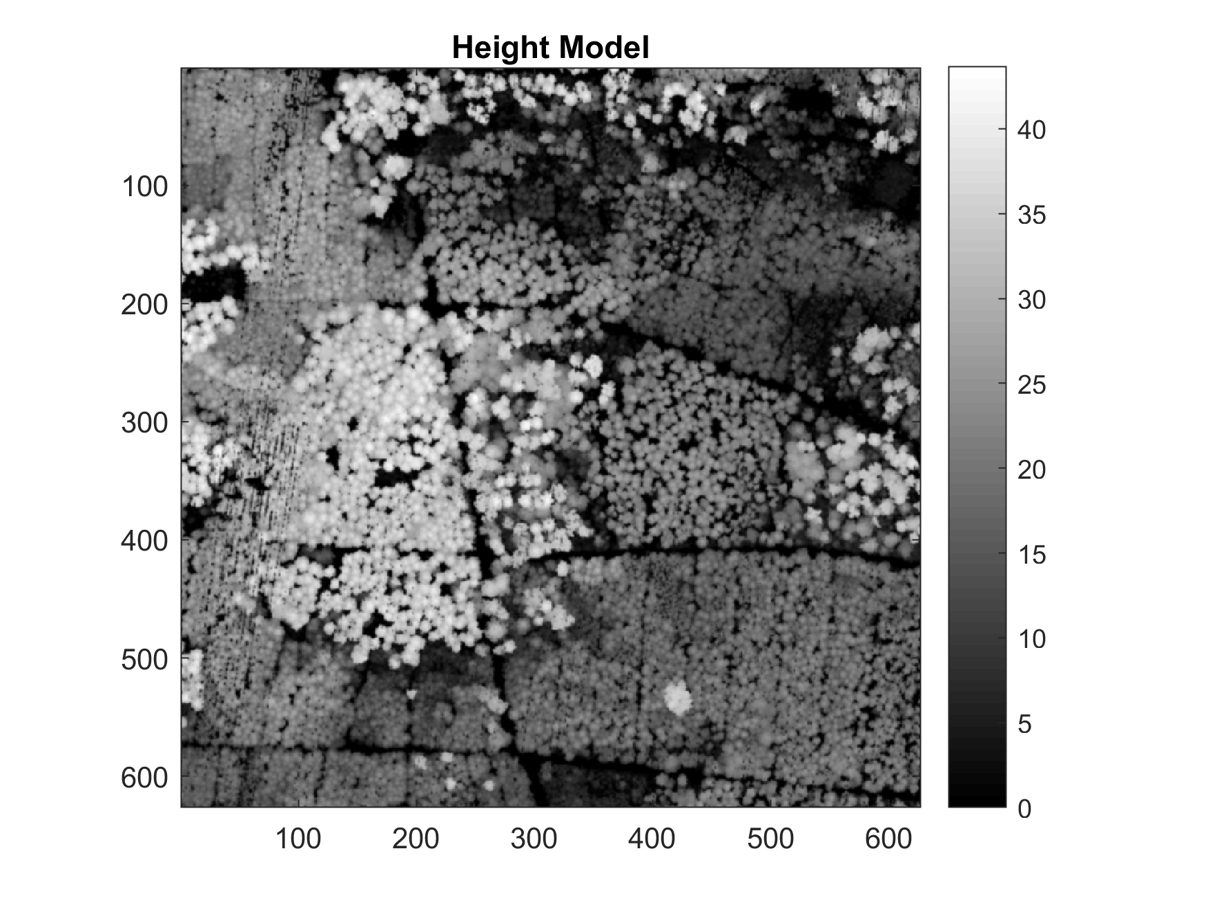
Step 2 - Computing a raster Canopy Height Model (CHM)
We now build 0.8 m resolution raster elevation models from the classified 3D point cloud using elevationModels():
cellSize = 0.8;
[models, refmat] = elevationModels([pc.record.x, pc.record.y, pc.record.z], ...
    pc.record.classification, ...
    'classTerrain', [2], ...
    'classSurface', [4,5], ...
    'cellSize', cellSize, ...
    'interpolation', 'idw', ...
    'searchRadius', inf, ...
    'weightFunction', @(d) d^-3, ...
    'smoothingFilter', fspecial('gaussian', [3, 3], 0.8), ...
    'outputModels', {'terrain', 'surface', 'height'}, ...
    'fig', true, ...
    'verbose', true);
Note that we have only used classes 4 (medium vegetation) and 5 (high vegetation) when computing the surface model (with the 'classSurface' parameter). We've also applied a 3x3 pixel Gaussian lowpass filter (with the 'smoothingFilter' parameter). The resulting CHM should look like this:
Step 3 - Exporting the elevation models to ARC/INFO ASCII grid file
To export the elevation models that were computed in the previous step to ARC/INFO ASCII grid files, use:
% export the Digital Terrain Model (DTM) to an ARC/INFO ASCII grid file
ASCwrite('zh_2014_a_dtm.asc', ...
    models.terrain.values, ...
    refmat, ...
    'precision', 2, ...
    'noData', -99999, ...
    'verbose', true);

% export the Digital Surface Model (DSM) to an ARC/INFO ASCII grid file
ASCwrite('zh_2014_a_dsm.asc', ...
    models.surface.values, ...
    refmat, ...
    'precision', 2, ...
    'noData', -99999, ...
    'verbose', true);

% export the Digital Height Model (DHM) to an ARC/INFO ASCII grid file
ASCwrite('zh_2014_a_dhm.asc', ...
    models.height.values, ...
    refmat, ...
    'precision', 2, ...
    'noData', -99999, ...
    'verbose', true);
Step 4 - Tree top detection
In this step, tree top (local maxima) detection is applied to the CHM. Following the method described in Chen et al. (2006), a power law was used to describe the relation between crown radius and height. Non-linear regression was applied to a set of (manually delineated) reference observations, to determine the parameter values of the power law model (see figure 2). Subsequently, the lower 95% prediction bound of the regression was used as the mimimum separation (merging) range (r) between tree tops as a function of their height (h):
$$\DeclareMathOperator*{\max}{max} r(h) = 0.28 \cdot h^{0.59} $$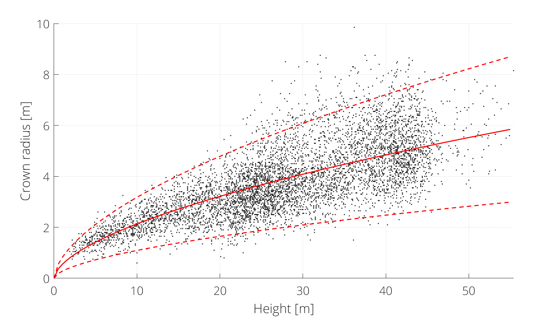
This model or any other, e.g. Popescu and Wynne (2004), can be specified for the 'searchRadius'parameter in the canopyPeaks() function:
[peaks_crh, ~] = canopyPeaks(models.height.values, ...
    refmat, ...
    'minTreeHeight', 2, ...
    'searchRadius', @(h) 0.28 * h^0.59, ...
    'fig', true, ...
    'verbose', true);
By modifing the 'searchRadius' parameter, you can adjust the tradeoff between the sensitivity (recall) and the reliability (precision) of the detection.
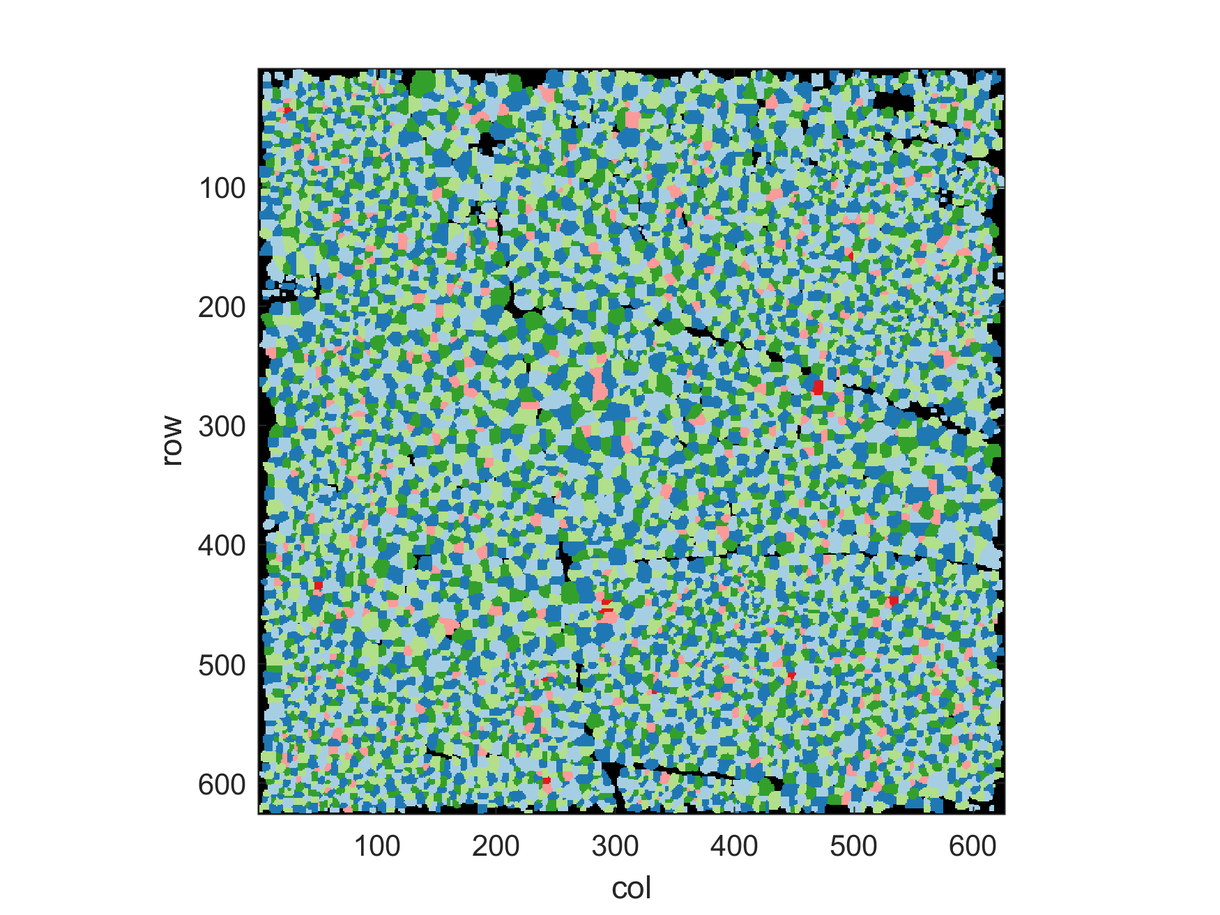
Step 5 - Marker controlled watershed segmentation
Using the previously computed CHM, tree top coordinates and boolean mask, we now compute the marker controlled watershed segmentation with treeWatershed():
[label_2d, colors] = treeWatershed(models.height.values, ...
    'markers', peaks_crh(:,1:2), ...
    'minHeight', 1, ...
    'removeBorder', true, ...
    'fig', true, ...
    'verbose', true);
Note that the "removeBorder" argument is set to true, to remove segments that touch the border of the image.
The resulting label matrix should look like this:
The interactive map below illustrates the detected tree top positions and edges of the watershed segmentation.
Step 6 - Computing segment metrics from the label matrix
From the labelled matrix, it is possible to compute a set of basic features (note that some of the metrics in regionprops() are currently only available in Matlab):
metrics_2d = regionprops(label_2d, models.height.values, ...
    'Area', 'Centroid', 'MaxIntensity');
Step 7 - Transferring 2D labels to the 3D point cloud
The next step is transferring the 2D labels and colors to the 3D point cloud:
idxl_veg = ismember(pc.record.classification, [4,5]);
% convert map coordinates (x,y) to image coordinates (column, row)
RC = [pc.record.x - refmat(3,1), pc.record.y - refmat(3,2)] / refmat(1:2,:);
RC(:,1) = round(RC(:,1)); % row
RC(:,2) = round(RC(:,2)); % column
ind = sub2ind(size(label_2d), RC(:,1), RC(:,2));
% transfer the label
label_3d = label_2d(ind);
label_3d(~idxl_veg) = 0;
[label_3d(label_3d ~= 0), ~] = grp2idx(label_3d(label_3d ~= 0));
% transfer the color index
color_3d = colors(ind);
color_3d(~idxl_veg) = 1;
% define a colormap
cmap = [0, 0, 0;
166,206,227;
31,120,180;
178,223,138;
51,160,44;
251,154,153;
227,26,28;
253,191,111;
255,127,0;
202,178,214;
106,61,154;
255,255,153;
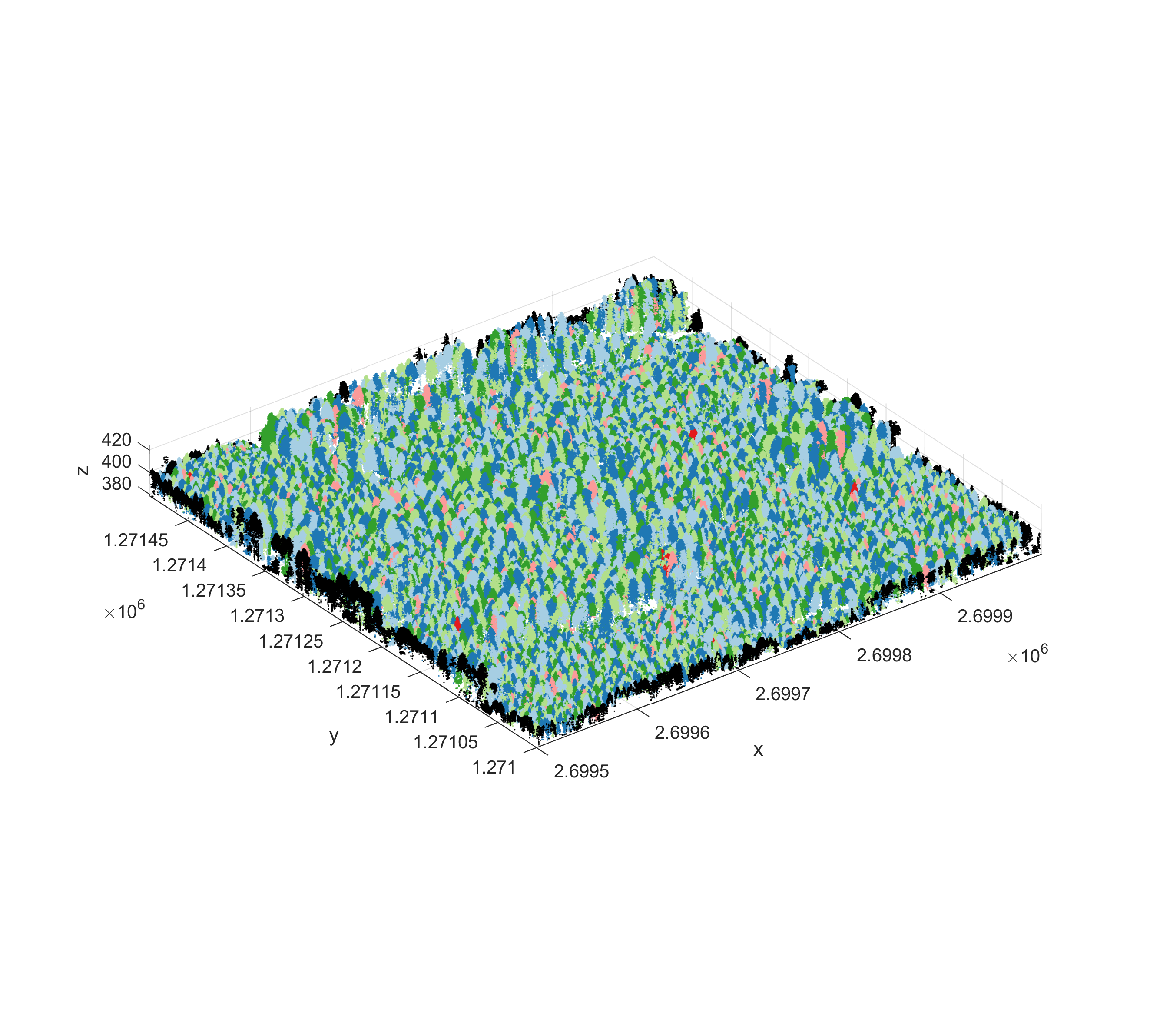
177,89,40] ./ 255;Step 8 - Plotting the colored points cloud
Octave users, due to 3D plotting performance issues, the display of large points clouds is currently discouraged.
To plot the complete colored point cloud, use:
if ~OCTAVE_FLAG

    figure('Color', [1,1,1])
    scatter3(pc.record.x(idxl_veg), ...
        pc.record.y(idxl_veg), ...
        pc.record.z(idxl_veg), ...
        6, ...
        color_3d(idxl_veg), ...
        'Marker', '.')
    axis equal tight
    colormap(cmap)
    caxis([1, size(cmap,1)])
    xlabel('x')
    ylabel('y')
    zlabel('z')

end
The result should look like this:
You can also plot any individual segment. For example segment n° 42:
if ~OCTAVE_FLAG

    idxl_sample = (label_3d == 42);
    figure
    scatter3(pc.record.x(idxl_sample), ...
        pc.record.y(idxl_sample), ...
        pc.record.z(idxl_sample), ...
        12, ...
        pc.record.intensity(idxl_sample), ...
        'Marker', '.');
    colorbar
    axis equal tight
    title('Return intensity')
    xlabel('x')
    ylabel('y')
    ylabel('z')

end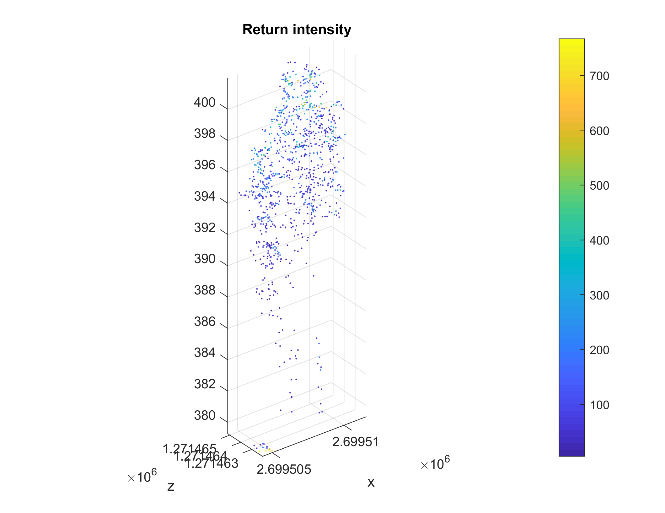
Step 9 - Computing segment metrics from the labelled point cloud
We now compute descriptive metrics directly from the point cloud for each segment using treeMetrics():
% compute metrics
[metrics_3d, fmt, idxl_scalar] = treeMetrics(label_3d, ...
    [pc.record.x, pc.record.y, pc.record.z], ...
    pc.record.intensity, ...
    pc.record.return_number, ...
    pc.record.number_of_returns, ...
    nan(length(pc.record.x), 3), ...
    models.terrain.values, ...
    refmat, ...
    'metrics', {'UUID', 'XPos', 'YPos', 'ZPos', 'H','BBOX2D', 'XCVH2D', 'YCVH2D', 'CVH2DArea', 'IQ50'}, ...
    'intensityScaling', true, ...
    'alphaMin', 1.5, ...
    'verbose', true);

% list field names
sfields = fieldnames(metrics_3d);
Step 10 - Exporting the segment metrics to a CSV file
The following illustrates how to export the segmentation metrics to a Comma Separated Values text file (.csv):
% IMPORTANT: adjust the path to the output CSV file (otherwise it will be created in the current folder)
fid = fopen('zh_2014_a_seg_metrics.csv', 'w+'); % open file
fprintf(fid, '%s\n', strjoin(sfields(idxl_scalar), ',')); % write header line
C = struct2cell(rmfield(metrics_3d, sfields(~idxl_scalar))); % convert structure to cell array
fprintf(fid, [strjoin(fmt(idxl_scalar), ','), '\n'], C{:}); % write cell array to CSV file
fclose(fid); % close file
After exporting the CSV file, you can try opening it in any text editor (e.g. Notepad++).
Step 11 - Exporting the segment points (and metrics) to a SHP file
To export the detected tree top points and associated metrics to an ESRI shapefile, we first make a copy (S1) of the metrics list, then remove all the non-scalar fields from it and finally add "Geometry", "X" and "Y" fields to it:
% duplicate the metrics structure (scalar fields only)
S1 = rmfield(metrics_3d, sfields(~idxl_scalar));

% add the geometry type
[S1.Geometry] = deal('Point');

% add the X coordinates of the polygons
[S1.X] = metrics_3d.XPos;

% add the Y coordinates of the polygons
[S1.Y] = metrics_3d.YPos;
Matlab users, the shapewrite() function included here is currently not compatible with Matlab. Please use the shapewrite() function from the official Matlab mapping toolbox instead.
Then use shapewrite() to write the SHP file:
% write non-scalar structure to SHP file
shapewrite(S1, 'zh_2014_a_seg_points.shp'); % IMPORTANT: adjust the path to the output SHP file (otherwise it will be created in the current folder)
clear S1
After exporting the SHP file, you can try opening it in any GIS software (e.g. Quantum GIS).
Step 12 - Exporting the segment polygons (and metrics) to a SHP file
To export the detected tree extent polygons and associated metrics to an ESRI shapefile, we first make a copy (S2) of the metrics list, then remove all the non-scalar fields from it and finally add "Geometry", "X", "Y" and "BoundingBox" fields to it:
% duplicate the metrics structure (scalar fields only)
S2 = rmfield(metrics_3d, sfields(~idxl_scalar));

% add the geometry type
[S2.Geometry] = deal('Polygon');

% add the X coordinates of the polygons
[S2.X] = metrics_3d.XCVH2D;

% add the Y coordinates of the polygons
[S2.Y] = metrics_3d.YCVH2D;

% add the bounding boxes [minX, minY; maxX, maxY]
[S2.BoundingBox] = metrics_3d.BBOX2D;
As previously, we then use shapewrite() to write the SHP file:
% write non-scalar structure to SHP file
shapewrite(S2, 'zh_2014_a_seg_polygons.shp'); % IMPORTANT: adjust the path to the output SHP file (otherwise it will be created in the current folder)
clear S2
Step 13 - Exporting the labelled and colored point cloud to a LAS 1.4 file
Finally, we export the colored point cloud to a LAS 1.4 file with LASwrite(). We start by duplicating the source file and adding the RGB records:
% duplicate the source file
r = pc;

% rescale the RGB colors to 16 bit range and add them to the point record
rgb = uint16(cmap(color_3d,:) * 65535);
r.record.red = rgb(:,1);
r.record.green = rgb(:,2);
r.record.blue = rgb(:,3);
We then add the "label" as an extra 32 bit record and add the metadata for this field in the Variable Length Records (cf. ASPRS LAS 1.4 specification for details about the meaning of the metadata fields):
% add the "label" field to the point record (as an uint32 field)
r.record.label = uint32(label_3d);

% add the "label" uint32 field metadata in the variable length records
% check the ASPRS LAS 1.4 specification for details about the meaning of the fields
% https://www.asprs.org/a/society/committees/standards/LAS_1_4_r13.pdf
vlr = struct;
vlr.value.reserved = 0;
vlr.value.data_type = 5;
vlr.value.options.no_data_bit = 0;
vlr.value.options.min_bit = 0;
vlr.value.options.max_bit = 0;
vlr.value.options.scale_bit = 0;
vlr.value.options.offset_bit = 0;
vlr.value.name = 'label';
vlr.value.unused = 0;
vlr.value.no_data = [0; 0; 0];
vlr.value.min = [0; 0; 0];
vlr.value.max = [0; 0; 0];
vlr.value.scale = [0; 0; 0];
vlr.value.offset = [0; 0; 0];
vlr.value.description = 'LABEL';

vlr.reserved = 43707;
vlr.user_id = 'LASF_Spec';
vlr.record_id = 4;
vlr.record_length_after_header = length(vlr.value) * 192;
vlr.description = 'Extra bytes';

% append the new VLR to the existing VLR
if isfield(r, 'variable_length_records')

    r.variable_length_records(length(r.variable_length_records)+1) = vlr;

else

    r.variable_length_records = vlr;

end
We also adjust the point data record format in the LAS header to support the RGB fields:
% if necessary, adapt the output record format to add the RGB channel
switch pc.header.point_data_format_id

    case 1 % 1 -> 3

        recordFormat = 3;

    case 4 % 4 -> 5

        recordFormat = 5;

    case 6 % 6 -> 7

        recordFormat = 7;

    case 9 % 9 -> 10

        recordFormat = 10;

    otherwise % 2,3,5,7,8,10

        recordFormat = pc.header.point_data_format_id;

end
Finally, we write the LAS file with LASwrite() and check that it has been correctly written with LASread():
% write the LAS 1.4 file
% IMPORTANT: adjust the path to the output LAS file
LASwrite(r, ...
    'zh_2014_a_ws_seg.las', ...
    'version', 14, ...
    'guid', lower(strcat(dec2hex(randi(16,32,1)-1)')), ...
    'systemID', 'SEGMENTATION', ...
    'recordFormat', recordFormat, ...
    'verbose', true);

% you can optionally read the exported file and check it has the
% RGB color and label records
% IMPORTANT: adjust the path to the input LAS file
r2 = LASread('zh_2014_a_ws_seg.las');
After exporting, you can try opening the LAS file in any appropriate CAD, GIS or 3D visualization software (e.g. Displaz, CloudCompare, FugroViewer).
References
- Chen, Q., Baldocchi, D., Gong, P., Kelly, M., 2006. Isolating Individual Trees in a Savanna Woodland Using Small Footprint Lidar Data. Photogrammetric Engineering and Remote Sensing 72, 923–932. https://doi.org/10.14358/PERS.72.8.923
- Kwak, D.-A., Lee, W.-K., Lee, J.-H., Biging, G.S., Gong, P., 2007. Detection of individual trees and estimation of tree height using LiDAR data. Journal of Forest Research 12, 425–434. https://doi.org/10.1007/s10310-007-0041-9
- Meyer, F., 1994. Topographic distance and watershed lines. Signal Processing, Mathematical Morphology and its Applications to Signal Processing 38, 113–125. https://doi.org/10.1016/0165-1684(94)90060-4
- Meyer, F., Beucher, S., 1990. Morphological segmentation. Journal of Visual Communication and Image Representation 1, 21–46. https://doi.org/10.1016/1047-3203(90)90014-M
- Pitkänen, J., Maltamo, M., Hyyppä, J., Yu, X., 2004. Adaptive methods for individual tree detection on airborne laser based canopy height model. International Archives of Photogrammetry, Remote Sensing and Spatial Information Sciences 36, 187–191.
- Popescu, S.C., Wynne, R.H., 2004. Seeing the trees in the forest: Using lidar and multispectral data fusion with local filtering and variable window size for estimating tree height. Photogrammetric Engineering and Remote Sensing 70, 589–604.
- Soille, P., 2013. Morphological image analysis: principles and applications. Springer Science & Business Media, Berlin, Germany.