Deciduous/evergreen foliage classification
Published: April 29, 2019 / Last updated: May 17, 2019
Tested on Matlab r2018b, GNU Octave 5.1.0
Introduction
This tutorial presents a simple approach to differentiate deciduous and evergreen foliage using the corrected return intensity of Airborne Laser Scanning (ALS) data. Foliage persistance maps can for example be useful to improve stem diameter prediction (by applying deciduous/evergreen specific allometric models) and for wildlife habitat modelling. This distinction is not to be confused with the distinction of broadleaf and coniferous, as some coniferous trees, such as larches, will shed their needles in automn while some broadleaf trees, such as hollies, will keep their leaves in winter.
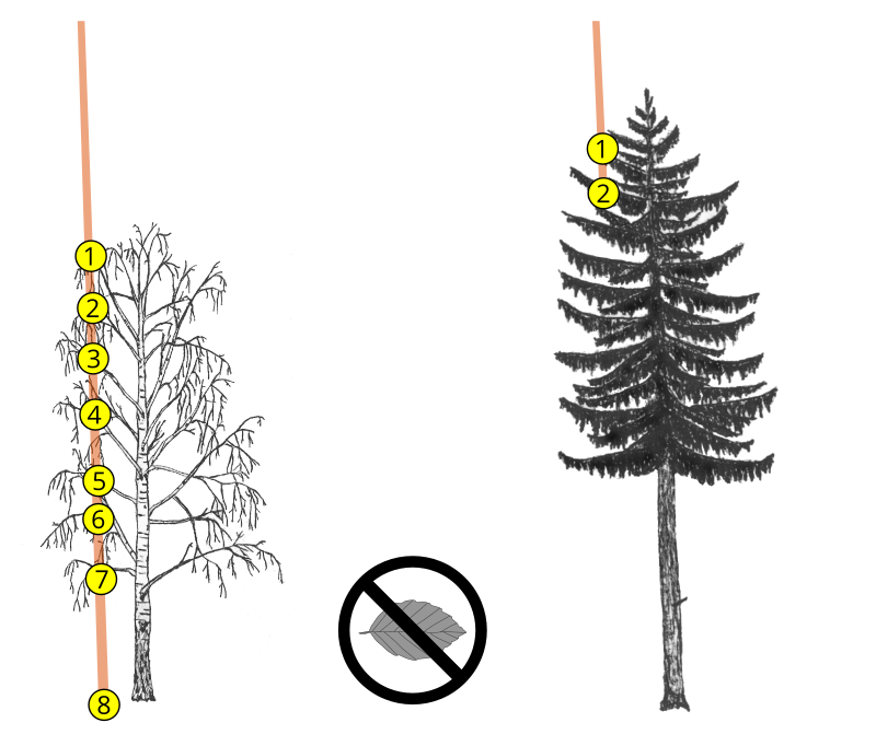
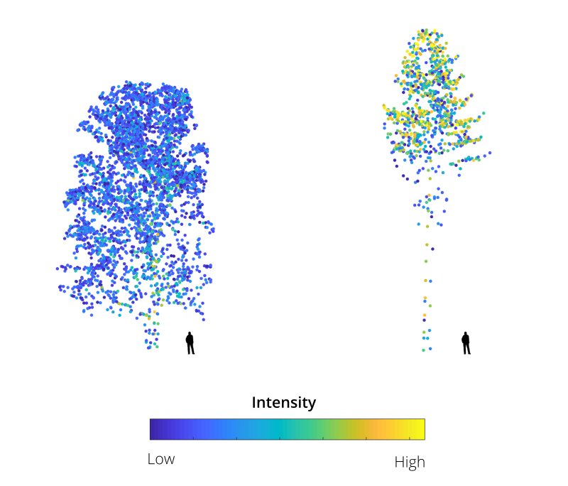
Dense foliage and large branches have a higher probability of completely intercepting the laser beam and generating single high intensity returns (see figures 1 and 2). Moreover, most LiDAR systems employ near infrared light which is strongly reflected by live foliage. Thus, ALS data acquired during leaf-off conditions can be readily used to differentiate deciduous and evergreen foliage. It has also been repeatedly demonstrated that the return intensity and ranking distributions of laser scans are important features to differentiate tree species (e. g. Liang et al., 2007; Ørka et al. 2009; Shi et al., 2018).
However, due to various instrumental and environmental effects, the raw intensity is generally inconsistent accross the surveyed area and cannot be directly used as a discriminative feature; it should first be corrected (Höfle and Pfeifer, 2007; Vain and Kaasalainen, 2011; Kashani et al., 2015). This can be a complex task, as the return intensity (a proxy of the power reflected by the target surface and received by the sensor) depends on parameters which can be difficult to estimate, as shown in the RaDAR/LiDAR range equation below:
$$P_r = \frac{D_{r}^2 \eta_{atm} \eta_{sys} \sigma P_t}{4 \pi R^4 \beta_{t}^2 }$$ $$\sigma = \frac{4 \pi}{\Omega} \rho A_t$$
where:
- \(P_r\) is the received power [W];
- \(P_t\) is the transmitted power [W];
- \(D_r\) is the aperture diameter [m];
- \(\eta_{atm}\) is the atmospheric transmittance;
- \(\eta_{sys}\) is the system transmittance;
- \(\sigma\) is the effective target cross-section [m2];
- \(R\) is the range from sensor to target [m];
- \(\beta_{t}\) is the width of the laser beam [m];
- \(\Omega\) is the scattering solid angle [sr];
- \(\rho\) is the reflectance of the target;
- \(A_t\) is the area of the target, i.e. area illuminated by the laser [m2].
The RaDAR/LiDAR range equation can be simplified, if we assume that the target is a Lambertian surface, that it has a scattering solid angle \(\Omega = \pi\) [sr] and that the entire laser beam is intercepted (Höfle and Pfeifer, 2007). Under these assumptions, the area of the target \(A_t\) and its effective cross section \(\sigma\) respectively become:
$$A_t = \frac{\pi R^2 \beta_{t}^2}{4}$$ $$\sigma = \pi \rho R^2 \beta_{t}^2 cos(\alpha)$$where:
- \(\alpha\) is the angle between the surface normal and the laser beam.
The received power \(P_r\) is then:
$$P_r = \frac{P_t D_{r}^2 \rho}{4 R^2} \eta_{atm} \eta_{sys} cos(\alpha)$$This shows that the range between the sensor and the target surface has a large influence (quadratic in this case) on the received power (received intensity). To compensate the decay of intensity with range, a correction can be applied, if the aircraft trajectory and return times are known, following for example the guidelines provided in Luzum et al. (2004):
$$I_{n} = I \cdot \left(\frac{R}{R_{ref}}\right)^2$$where:
- \(I_n\) is the range normalized intensity;
- \(I\) is the raw intensity;
- \(R\) is the range from sensor to target [m];
- \(R_{ref}\) is an arbitrary constant reference range (e. g. 1000 m).
Altough none of the modelling assumptions used above are realistic when dealing with complex objects such as trees, this simple range correction may help homogenise intensity values accross the dataset. ALS post-processing software generally offer the possibility to apply some form of intensity correction. Riegl's RiProcess software, for example, lets you export either the amplitude (range dependent value) or a range independant value which they call reflectance to the "intensity" field in LAS files (Riegl Laser Measurement Systems, 2017). In this tutorial, we will use data acquired over the state of Geneva (Switzerland) in February 2017 (leaf-off conditions) with the Riegl LMS-Q1560 sensor. The data is openly available from Geneva's Official Geodata Portal. The intensity stored in the LAS file is the reflectance (i.e. range independent value) scaled to a 16 bit range (0-65535), so no further range correction is required. If you would like to apply the approach illustrated in this tutorial to other ALS datasets, you should first inquire if and how the intensity has been processed.
A small forest located about 10 km to the North of Geneva city (see map below) will serve as our study case. Within this area, the main tree species are pedunculate oak (Quercus robur) and Scots pine (Pinus sylvestris).
Setup
- Download and uncompress the Digital Forestry Toolbox (DFT) Zip or Tar archive
- Download the ge_2017_a.laz file from the DFT Zenodo repository and uncompress it with LASzip
- Start Matlab/Octave
- Delete any previous versions of the toolbox
- Add the DFT folders to the Matlab/Octave search path using
addpath(genpath('path to DFT main folder')) - Open
dft_tutorial_4.m(located in the tutorials folder)
Step 1 - Reading the LAS file
We start by reading the LAS file using LASread():
pc = LASread('ge_2017_a.las');

xyz = [pc.record.x, pc.record.y, pc.record.z];
intensity = double(pc.record.intensity);
Note that you may have to adjust the file path in the code above, depending on where you are storing the LAS file. Also note that the point classification uses the following scheme:
| Class | Description |
|---|---|
| 0 | Created, never lassified |
| 1 | Unclassified |
| 2 | Terrain |
| 3 | Low vegetation (< 50 cm) |
| 5 | High vegetation (≥ 50 cm) |
| 6 | Buildings |
| 7 | Outliers and incorrect measurements (Low noise) |
| 9 | Water |
| 13 | Bridges |
| 15 | Terrain (additional points) |
| 16 | Outliers and incorrect measurements (High noise) |
| 19 | Points measured outside of the area of interest (unclassified) |
Step 2 - Compute raster elevation models
In this step, we compute 0.5x0.5 m raster elevation models, using the elevationModels() function:
cellSize = 0.5;
[models, refmat] = elevationModels([pc.record.x, pc.record.y, pc.record.z], ...
    pc.record.classification, ...
    'classTerrain', [2, 9, 16], ...
    'classSurface', [3, 4, 5], ...
    'cellSize', cellSize, ...
    'closing', 3, ...
    'smoothingFilter', [], ...
    'outputModels', {'terrain', 'surface', 'height'}, ...
    'fig', true, ...
    'verbose', true);

% convert map coordinates to image coordinates
[nrows, ncols] = size(models.terrain.values);
P = [pc.record.x - refmat(3,1), pc.record.y - refmat(3,2)] / refmat(1:2,:);
row = round(P(:,1));
col = round(P(:,2));
ind = sub2ind([nrows, ncols], row, col);
Step 3 - Filter the canopy points
We now create a filter which selects only high vegetation points located in the top highest 1 m section of the canopy:
idxl_veg = ismember(pc.record.classification, [4,5]);

z_margin = 1;
idxl_canopy = pc.record.z >= (models.surface.values(ind) - z_margin);
idxl_filter = idxl_veg & idxl_canopy;
Step 4 - Compute an intensity map
We create the intensity map by averaging the intensity of the canopy points located in each of the raster cells:
% computing the mean using sum() and numel() is faster than using mean() in accumarray
I = accumarray([row(idxl_filter), col(idxl_filter)], double(pc.record.intensity(idxl_filter)), [nrows, ncols], @sum, 0) ./ ...
    accumarray([row(idxl_filter), col(idxl_filter)], double(pc.record.intensity(idxl_filter)), [nrows, ncols], @numel, 1);
The resuling raster can be displayed with:
figure
imagesc(I);
axis equal tight
colorbar
caxis(quantile(I(:), [0.02, 0.98]))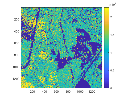
Notice that the resulting intensity map is somewhat noisy due to the presence of small high intensity spots (near tree stems). You can optionally export the intensity map to an ARC/INFO ASCII grid file with the ASCwrite() function:
ASCwrite('ge_2017_a_intensity.asc', ...
    I, ...
    refmat, ...
    'precision', 2, ...
    'noData', -99999, ...
    'verbose', true);
Step 5 - Segmentation
One simple approach to smooth the intensity map we obtained in the previous step is to apply segmentation and average the intensity in each segment. We will only illustrate the Simple Linear Iterative Clustering (SLIC) proposed by Achanta et al. (2012), but other segmentation algorithms such as the marker controlled watershed segmention (cf. tutorial 2) could be used as well. SLIC is modified K-means algorithm, where the relative importance of spatial separation and color (or grayscale) similarity of clusters can be controlled with a compacity parameter. Matlab users who have access to the image processing toolbox can use the superpixels() function. Octave users (or Matlab users who dot not have the image processing toolbox) have to compile the SLICmex.c function provided by Achanta et al. (and included in the external functions directory of the Digital Forestry Toolbox), by typing the following line in the command window:
mex slicmex.cThen run the following code:
segmentation = 'slic'; % specify 'slic' or 'watershed'

switch segmentation

    case 'slic' % Superpixel segmentation

        % rescale values to an 8 bit range (0-255)
        I_n = (I - quantile(I(:), 0.02)) ./ diff(quantile(I(:), [0.02, 0.98]));
        I_n = uint8(I_n * 255);

        % before running slicmex, you have to compile it with the following command:
        % mex slicmex.c
        r = 2.5; % target radius of one superpixel (in map units)
        a = pi*r^2; % target area of one superpixel (in map units)
        n_superpixels = round(nrows * ncols * cellSize^2 / a); % number of superpixels
        [L, nlabels] = slicmex(I_n, n_superpixels, 100);

        % Note: Matlab users who have the "image processing" toolbox can also use the superpixels() function
        % [L, nlabels] = superpixels(I_n, n_superpixels, 'Compactness', 75);

    case 'watershed' % Marker controlled watershed segmentation

        [peaks_crh, ~] = canopyPeaks(models.height.values, ...
            refmat, ...
            'minTreeHeight', 2, ...
            'smoothingFilter', fspecial('gaussian', [3 3], 1), ...
            'searchRadius', @(h) 0.28 * h^0.59, ...
            'fig', false, ...
            'verbose', true);

        [L, ~] = treeWatershed(models.height.values, ...
            'markers', peaks_crh(:,1:2), ...
            'minHeight', 1, ...
            'removeBorder', false, ...
            'fig', false, ...
            'verbose', true);

end
The interactive map below illustrates the intensity map (in grayscale) and the superpixel boundaries (in yellow) obtained with the SLIC approach. Try using the transparency slider on the map to visualize the overlap between the superpixels and underlying canopy extent.
Step 6 - Compute segment level intensity
We now compute the mean intensity and maximum height of each segment with:
I_s = accumarray(L(:)+1, I(:), [nrows*ncols,1], @nanmean, nan);
I_s = I_s(L+1);
H_s = accumarray(L(:)+1, models.height.values(:), [nrows*ncols,1], @nanmax, single(nan));
H_s = H_s(L+1);
We then remove segments with a maximum height smaller than 3 m and those containing only null intensity values:
h_min = 3;
I_s(H_s <= h_min) = nan;

I_s(I_s == 0) = nan;
Step 7 - Create a classification map
We start by examining the distribution of intensity values with a histogram:
figure
hist(I_s(~isnan(I_s)), 100)
xlabel('intensity')
ylabel('count')
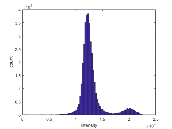
Notice the bimodal distribution, with two peaks around 12'000 and 20'000. To separate non-tree, deciduous and evergreen areas, we can split the values into low (< 7500), medium (≥ 7500 to < 17'000) and high (≥ 17'000) intensity categories with the histc() function:
[~, C] = histc(I_s(:), [7500, 17000, inf]);We then reshape the intensity categories vector into an array and plot it:
C = reshape(C, nrows, ncols);
figure
imagesc(C)
axis equal tight
Step 8 - Filter out small patches
To remove small patches in the evergreen category (C = 2), we apply morphological reconstruction to the category 2 boolean image, using a morphological erosion (with a disk shaped window with a 3 pixel radius) as the marker:
se = strel("disk", 3, 0); % circular structuring element with a radius of 3 pixels
J = imreconstruct(imerode(C == 2, se), C == 2);
C(J ~= (C == 2)) = 1;
Finally, you can optionally export the category map to an ARC/INFO ASCII grid file with the ASCwrite() function:
ASCwrite('ge_2017_a_class.asc', ...
    C, ...
    refmat, ...
    'precision', 0, ...
    'noData', -99999, ...
    'verbose', true);
After exporting the map, you can try opening it in any GIS software (e.g. Quantum GIS). The interactive map below illustrates the categorical map overlayed on a leaf-off orthoimage of the same area (try moving the transparency slider to compare it with the orthoimage). Note that the features in the LiDAR derived map and in the orthoimage do not overlap perfectly. This is due to the orthorectification process which used a terrain model instead of a surface model.
References
- Achanta, R., Shaji, A., Smith, K., Lucchi, A., Fua, P., Süsstrunk, S., 2012. SLIC Superpixels Compared to State-of-the-Art Superpixel Methods. IEEE Transactions on Pattern Analysis and Machine Intelligence 34, 2274–2282. https://doi.org/10.1109/TPAMI.2012.120
- Höfle, B., Pfeifer, N., 2007. Correction of laser scanning intensity data: Data and model-driven approaches. ISPRS Journal of Photogrammetry and Remote Sensing 62, 415–433. https://doi.org/10.1016/j.isprsjprs.2007.05.008
- Kashani, A.G., Olsen, M.J., Parrish, C.E., Wilson, N., 2015. A Review of LIDAR Radiometric Processing: From Ad Hoc Intensity Correction to Rigorous Radiometric Calibration. Sensors 15, 28099–28128. https://doi.org/10.3390/s151128099
- Liang, X., Hyyppä, J., Matikainen, L., 2007. Deciduous-coniferous tree classification using difference between first and last pulse laser signatures. International Archives of Photogrammetry, Remote Sensing and Spatial Information Sciences 36, 253–257.
- Luzum, B., Starek, M., Slatton, K.C., 2004. Normalizing ALSM intensities (No. Rep_2004-07-01), Geosensing Engineering and Mapping (GEM) Center. Civil and Coastal Engineering Department, University of Florida, Gainesville, FL, USA.
- Ørka, H. O., Næsset, E., Bollandsås, O. M., Jun. 2009. Classifying species of individual trees by intensity and structure features derived from airborne laser scanner data. Remote Sensing of Environment 113 (6), 1163–1174.
- Riegl Laser Measurement Systems, 2017. LAS Extrabytes Implementation in RIEGL Software. Riegl Laser Measurement Systems GmbH, Horn, Riedenburgstrasse 48, Austria.
- Shi, Y., Wang, T., Skidmore, A. K., Heurich, M., Mar. 2018b. Important LiDAR metrics for discriminating forest tree species in Central Europe. ISPRS Journal of Photogrammetry and Remote Sensing 137, 163–174.
- Vain, A., Kaasalainen, S., 2011. Correcting airborne laser scanning intensity data. INTECH Open Access Publisher.